Imagine we design a test to detect a disease. In the graph below are 500 patients.

• Some patients have a positive test result and also have the disease; this is a True Positive (TP).
• Some patients don’t have the disease but nevertheless have a positive test result; this is a False Positive (FP).
• Most patients do not have the disease and, accordingly, have a negative test result; this is a True Negative (TN).
• A few patients do have the disease, but, unfortunately, had a negative test result; this is a False Negative (FN).

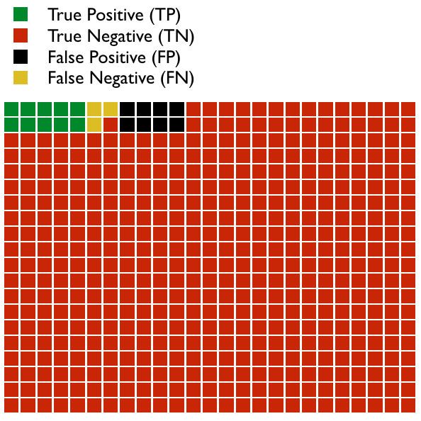
In this example, we see that: TP = 10, FP = 8, TN = 479, and FN = 3. In this population, the Prevalence of the disease is = (TP + FN)/total number, which = 13/500 or 2.6%. Don’t confuse prevalence with Incidence, which is the number of new cases of the disease in a given amount of time.

We can talk about how well our test works in a variety of different ways. Some of these terms are mistakenly interchanged and can be grossly misinterpreted if you don’t understand them correctly. Let’s look at each briefly (please don’t get overwhelmed by the math, and if you do, skip to the end and read the take away points):

• Sensitivity (True Positive Rate) = TP/P = TP/(TP+FN) = 10/(10+3) = 5/8 = 76.9%
  • Thinking of sensitivity as the true positive rate is more intuitive. It means that 76.9% of patients with the disease were correctly identified as having it.
• Specificity (True Negative Rate) = TN/N = TN/(TN+FP) = 479/(479+8)=479/487 = 98.4%
  • Again, specificity makes more sense as the true negative rate. It means that 98.4% of people who do not have the disease were correctly identified as not having it.
• Precision (Positive Predictive Value, PPV) = TP/(TP+FP) = 10/(10+8) = 55.6%
  • The PPV is the proportion of patients with a positive test who actually have the disease. In this case, if your test is positive, you have a 55.6% chance of having the disease. Notice the difference between PPV and sensitivity.
• Negative Predictive Value (NPV) = TN/(TN+FN) = 479/(479+3) = 99.4%
  • The NPV is the proportion of patients with a negative test who actually do not have the disease. In this case, if your test is negative, you have a 99.4% chance that you do not have the disease. Notice the difference between NPV and specificity.
• False Positive Rate = 1 – specificity = 1.6%
  • 1.6% of people who do not have the disease were incorrectly identified as having the disease.
• False Negative Rate = 1 – sensitivity = 23.1%
  • 23.1% of people who have the disease were incorrectly identified as not having the disease.
• False Discovery Rate = 1 – precision = 44.4%
  • 44.4% of people with a positive result do not have the disease (this is the proportion of positive results that are false positives).
• Accuracy = (TP+TN)/(TP + FP + FN + TN) = 479+10/500 = 97.8%
  • This term is very misleading. It is simply the proportion of true results out of all results, both true positives and true negatives. So this test is 97.8% accurate. This would obviously be the number we would use to sell our new test to doctors! Yet, it is misleading. The PPV (55.6%) and the NPV (99.4%) are the most clinically useful results. But since most results are negative, then the accuracy of the test (which lies between the PPV and the NPV) is very close to and approaching the NPV.

Note: The popular mnemonics SPIN and SNOUT that med students use to remember specificity and sensitivity are misleading. SPIN states that a highly SPecific test (when positive) rules IN a disease, while SNOUT states that a highly SeNsitive test, when negative, rules OUT a disease. This is misleading because both sensitivity and specificity influence the utility of a test to predict or exclude a disease, as we will see next.

There are two additional important terms to define:

• Positive Likelihood Ratio (or LR+) = Sensitivity/(1-Specificity) = 0.769/(1-0.984) = 48
  • This is the probability of a person who has the disease testing positive, divided by the probability of a person who doesn’t have the disease testing positive.
• Negative Likelihood Ratio (or LR-) = (1-Sensitivity)/Specificity = (1-0.769)/0.984 = 0.23
  • This is the probability of a person who has the disease testing negative, divided by the probability of a person who does not have the disease testing negative.

All of the characteristics of our test that we have discussed so far are independent of the prevalence. We have not considered the prevalence of the disease in any of our calculations. We know what the prevalence of the disease in the 500 patients we studied is, but this might not be the actual prevalence in the population as a whole or in our population of patients that we see, or it may not be the probability of an individual patient sitting in front of us.

The most useful characteristics, clinically, of the test that we have learned about so far are the PPV and the NPV. These tell us what we need to know when the probability of the disease is equal to the prevalence of the disease in our study. But, unfortunately, they do not tell us how the test will perform in the real world. Clinically, when we order a test, the questions we should ask ourselves are, first, How likely is it that my patient has the disease? and, secondly, after the test result comes back, How likely is it that my patient has the disease now that I know the result of the test? These questions relate to the pre-test probability and the post-test probability. This process is the fundamental process that should be utilized when making clinical and diagnostic decisions, and is part of what we refer to as Bayesian Inference.

How do we determine the pre-test probability?

• It may be the known prevalence of the disease in a population; for example, the rate of breast cancer in white women in their 40s, or the rate of HIV in patients who have tuberculosis, or the rate of fetal Down Syndrome in 40 year-old pregnant women.
• It may be based on the results of a previous test, that is, the post-test probability of a test already performed.
• It may be a rough estimation based on clinical experience and the history and physical. This is often very imprecise, and may be divided into low, medium, or high probability. It can be more precise; for example, when based on clinical tools, like the Centor Criteria for strep throat. The reliability of these clinical estimates improves the more we learn about the relative risks of various risk factors for the disease. This is the clinical process we used in How Do I Diagnosis Ruptured Membranes? Bayesian Statistics at its Best.

Once we know the pre-test probability, and we have decided that a particular test is likely to be useful, we can then determine the post-test probability.

How do we determine the post-test probability?

• If the pre-test probability is the same as the prevalence of the disease used in the study (for our test, the prevalence was 2.6%), then the positive post-test probability is equal to the PPV, which was 55.6% for our test. However, it is rare, in the real world, that the patient is front of you has the same probability of having the disease as the prevalence used in the study.
• Thus, the more useful method of calculating the post-test probability is to use the pre-test probability and the likelihood ratio.
  • Positive post-test probability = (post-test odds)/(post-test odds +1)
    • Post-test odds = pretest odds X positive likelihood ratio
    • Pre-test odds = pre-test probability / (1 – pretest probability)
  • Thus, in our example, if we use the prevalence of the disease as our pretest probability (2.6%):
    • pre-test odds = 0.026 / (1 – 0.026) = 0.0267
    • post-test odds = 0.0267 x 48 = 1.28
    • positive post-test probability = 1.28/(1.28+1) = 56%
  • So using this method, with some rounding errors, we see that our post-test probability is roughly the same as the PPV for patients in whom we assume a pre-test probability equal to the prevalence of the disease.
  • What if we did not assume the same prevalence? What if, instead, we assumed that the patient had a 60% pre-test probability, based on risk factors, history, physical exam, and preliminary evaluations? Then,
    • pre-test odds = 0.6 / (1 – 0.6) = 1.5
    • post-test odds = 1.5 x 48 = 72
    • positive post-test probability = 72/(72+1) = 98.6%
  • So the same test has much more clinical value if the pre-test probability is high, compared to when it is lower.
  • What if the pre-test probability were lower, say 1/1000?
    • pre-test odds = 0.001 / (1 – 0.001) = 0.0001001
    • post-test odds =  0.0001001 x 48 = 0.0048048
    • positive post-test probability = 0.0048048/(0.0048048+1) = 0.478%

Here is the vast importance of Bayesian Inference in clinical reasoning: The same test, with the same performance characteristics, has two entirely different meanings (post-test probabilities) when applied to patients with different pre-test probabilities.

Take Away Points

When tests are arbitrarily applied to patients without knowledge of the pre-test probabilities of the condition being test for, then serious diagnostic mistakes happen. For example, ordering a screening CBC on an asymptomatic patient; if the test reveals some abnormality, it will be very unlikely that the result has any clinical meaning. Tests perform differently when applied to different populations or to patients with different presentations.

I have found that clinicians struggle with this idea almost more than any other concept in medicine. It seems so non-intuitive. Let me try an example:

Imagine that we develop a test to determine if a man is a hipster or not. Our test is, “Is he a white male with a full, thick beard?” We determine the sensitivity and specificity for this by sampling 10,000 men randomly across the country. We find that our test is 85% sensitive and 90% specific for being a hipster. From this, we can determine PPV and NPV and all of the other stats we have looked at so far. But we need to use this test clinically and understand how to interpret a positive result. Will the post-test probability for this test be the same if we apply it at a Starbucks in Seattle as compared to a bar at a lumberjack camp outside of Juneau, Alaska? Clearly not. This reflects the fact that, although we can determine a true prevalence of being a hipster, nevertheless hipsters are not distributed equally throughout America. We do not use tests in a vacuum. We use them with some prior knowledge and that prior knowledge (pre-test probability) affects the test’s meaning.

For more reading, try:

• Diagnostics and Likelihood Ratios Explained
• Students 4 Best Evidence: EBM at the Bedside
• And here is a calculator to do the work for you: Post-test Probability Calculator