

If you torture data for long enough, it will confess to anything. – Ronald Harry Coas
Imagine that you’ve just read a study in the prestigious British Medical Journal that concludes the following:
Remote, retroactive intercessory prayer said for a group is associated with a shorter stay in hospital and shorter duration of fever in patients with a bloodstream infection and should be considered for use in clinical practice.
Specifically, the author randomized 3393 patients who had been hospitalized for sepsis up to ten years earlier to two groups: the author prayed for one group and did not pray for the other. He found that the group he prayed for was more likely to have had shorter hospital stays and a shorter duration of fever. Both of these findings were statistically significant, with a p value of 0.01 and 0.04, respectively. So are you currently praying for the patients you hospitalized 10 years ago? If you aren’t, some “evidence-based medicine” practitioners (of the Frequentist school) might conclude that you are a nihilist, choosing to ignore science. But I suspect that even after reading the article, you are probably going to ignore it. But why? How do we know if a study is valid and useful? How can we justify ignoring one article while demanding universal adoption of another, when both have similar p values?
Let’s consider five steps for determining the validity of a study.
1. How good is the study?
Most published studies suffer from significant methodological problems, poor designs, bias, or other problems that may make the study fundamentally flawed. If you haven’t already, please read How to Read A Scientific Paper for a thorough approach to this issue. But if the paper looks like a quality study that made a statistically significant finding, then we must address how likely it is that this discovery is true.
2. What is the probability that the discovered association (or lack of an association) is true?
Of the many things to consider when reading a new study, this is often the hardest question to answer. The majority of published research is wrong; this doesn’t mean, however, that (in most cases) a scientific, evidence-based approach is still not the best way to determine how we should practice medicine. The fact that most published research is wrong is not a reason to embrace anecdotal medicine; almost every anecdotally-derived medical practice has been or will be eventually discredited.
It does mean, though, that we have to do a little more work as a scientific community, and as individual clinicians, to ascertain what the probability of a finding being “true” or not really is. Most papers that report something as “true” or “significant” based on a p value of less than 0.05 are in error. This fact was popularized in 2005 by John Ioannidis, whose paper has inspired countless studies and derivative works analyzing the impact of this assertion. For example,
- This 2012 report, published in Nature, found that only 6 of 53 high-profile cancer studies could be replicated in repeat experiments.
- This Frequentist paper, published in 2013, attempting to attack the methods of Ionnidis, still estimated that 14% of 5,322 papers published in the five largest medical journals contained false findings. This paper’s estimate is limited because it assumes that no study was biased and that authors did not manipulate p values, and it was further limited because it represents only papers published in the premier journals (presumably most poorer quality papers are published elsewhere as well as most preliminary and explorative studies).
- This paper, published in JAMA in 2005, found that of 49 highly cited articles, only 2o had results that were replicated while 7 were explicitly contradicted by future studies. Others suffered from differences in the size of the reported effect in subsequent studies.
- In 2015, Nature reported that only 39 of 100 psychology studies could be reproduced.
- This paper, published in 2010, found that 10 of 18 genetic microarray studies could not be replicated.
- RetractionWatch provides this overview of how many studies turn out to be untrue.
- This article in The Economist and this YouTube video both offer excellent visual explanations of these problems.
- Maybe the very best article about the scope of the problem is here, at fivethirtyeight.
P-hacking, fraud, retractions, lack of reproducibility, and just honest chance leading to the wrong findings; those are the some of the problems, but what’s the solution? Bayesian inference.
Bayes’ Theorem states:

This equations states that the probability of A given B is equal to the probability of B given A times the probability of A, divided by the probability of B. Don’t be confused. Let’s restate this for how we normally use it in medicine. What we care about is the probability that our hypothesis, H, is true, whatever our hypothesis might be. We test our hypothesis with a test, T; this might be a study, an experiment, or even a lab test. So here we can substitute those terms:

Normally, when we do a test (T), the test result is reported as the probability that the test or study (or the data collected in the study) fits the hypothesis. This is P(T | H). It assumes that the hypothesis is true, and then tells us the probability that the observed data would make our test or study positive (typically taken as a p value < 0.05). But this isn’t helpful to us. I want to know if my hypothesis is true, not just if the data collected and the tests performed line up with what I would expect to see if my hypothesis were true.
Frequentist statistics, the traditionally taught theory of statistics mostly used in biologic sciences, is incapable of answering the question, “How probable is my hypothesis?” Confused by this technical point, most physicians and even many research scientists wrongly assume that when a test or study is positive or “statistically signficant,” that the hypothesis being tested is validated. This misassumption is responsible for the vast majority of the mistakes in science and in the popular interpretation of scientific articles.
Pause…
If Frequentism versus Bayesianism is confusing (I’m sure it probably is), let’s simplify it.
Imagine that you are standing in a room and you hear voices in the next room that sound exactly like Chuck Norris talking to Jean-Claude van Damme. Thrilled, you quickly record the voices. You develop a hypothesis that Chuck and van Damme are in the room next door to you. You use a computer to test whether the voices match known voice samples of the two martial artists. The computer test tells you that the voices are nearly a perfect match, with a p value of < 0.0001. This is what Frequentist statistical methods are good at. This statistical approach tells you the chance that the data you observed would exist if your hypothesis were true. Thus, it tells you the probability of the voice pattern you observed given that the JCVD and Chuck are in the room next door; that is, the probability of the test given the hypothesis, or P(T | H).
But it doesn’t tell you if your hypothesis is true. What we really want to know is the probability that Chuck and the Muscles from Brussels are in the room next door, given the voices you have heard; that is, the probability of the hypothesis given the test, or P(H | T). This is the power of Bayesian inference, because it allows us to consider other information that is beyond the scope of the test, like the probability that the two men would be in the room in the first place compared to the probability that the TV is just showing a rerun of The Expendables 2.
Bayes tells us the probability of an event based on everything we know that might be related to that event, and it is updated as new knowledge is acquired.
Frequentism tells us the probability of an event based on the limit of its frequency in a test. It does not allow for the introduction of prior knowledge or future knowledge.
Our brains naturally work using Bayesian-like logic so it should come naturally.
Resume…
So we need Bayes to answer the question of how probable our hypothesis actually is. More specifically, Bayesian inference allows us to change our impression of how likely something is based on new data. So, at the start, we assume that a hypothesis has a certain probability of being true; then, we learn new information, usually from experiments or studies; then, we update our understanding of how likely the thing is to be true based on this new data. This is called Bayesian Updating. As I said, the good news is, you are already good at this. Our brains are Bayesian machines that continuously learn new information and update our understanding based on what we learn. This is the same process we are supposed to be using to interpret medical tests, but in the case of a scientific study, instead of deciding if a patient has a disease by doing a test, we must decide if a hypothesis is “true” (at least highly probable) based on an experimental study.
Let’s see how Bayesian inference helps us determine the true rates of Type I and Type II errors in a study.
Type I and Type II Errors
Scientific studies use statistical methods to test a hypothesis. If the study falsely rejects the null hypothesis (that there is no association between the two variables), then that is called a Type I Error, or a false positive (since it incorrectly lends credence to the alternative hypothesis). If there is an association that is not detected, then this is called a Type II Error, or false negative (since it incorrectly discounts the alternative hypothesis).
We generally accept that it’s okay to be falsely positive about 5% of the time in the biological sciences (Type 1 Error). This rate is determined by alpha, usually set to 0.05; this is why we generally say that anything with a p value < 0.05 is significant. In other words, we are saying that it is okay to believe a lie 5% of the time.
The “power” of a study determines how many false negatives there will be. A study may not have been sufficiently “powered” to find something that was actually there (Type II Error). Power is defined as 1 – beta; most of the time, beta is 0.2, and this would mean that a study is likely to find 80% of true associations that exist. In other words, we miss something we wanted to find 20% of the time.
In order for the p value to work as intended, the study must be powered correctly. Too few or too many patients in the study creates a problem. So a power analysis should performed before a study is conducted to make sure that the number of enrolled subjects (the n) is correct.
Most people who have taken an elementary statistics course understand these basic principles and most studies at least attempt to follow these rules. However, there is a big part still missing: not all hypotheses that we can test are equally likely, and that matters.
For example compare these two hypotheses: ‘Cigarette smoking is associated with development of lung cancer’ versus ‘Listening to Elvis Presley music is associated with development of brain tumors.’ Which of these two hypotheses seems to be more likely, based on what we already know, either from prior studies on the subject or studies related to similar subject matter? Or if there are no studies, based on any knowledge we have, including our knowledge of basic sciences?
We need to understand the pre-study probability that the hypothesis is true in order to understand how the study itself affects the post-study probability. This is the same skill set we use when we interpret clinical tests: the test is used to modulate our assigned pretest probability and to generate a new posttest probability (what Bayesians call the posterior probability). So, too, a significant finding (or lack of a significant finding) is used to modulate the post-study probability that a particular hypothesis is true or not true.
Let’s say that we create a well-designed study to test our two hypotheses (the cigarette hypothesis and the Elvis hypothesis). It is most likely that the cigarette hypothesis will show a positive link and the Elvis hypothesis will not. But what if the cigarette hypothesis doesn’t find a link for some reason? Or the Elvis hypothesis does show a positive link? Do we allow these two studies to upend and overturn everything we currently know about the subjects? Not if we use Bayesian inference.
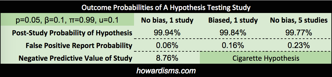
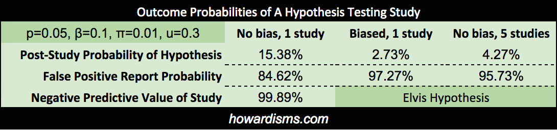
I’m not sure what the pre-study probabilities that these two hypothesis are true should be, but I would guess that there is a 99% chance, based on everything we know, that cigarette smoking causes lung cancer, and about a 1% chance that listening to Elvis causes brain tumors. Let’s see what this means in real life.
We can actually calculate how these pre-study probabilities affect our study, and how our study affects our assumptions that the hypotheses are true. Assuming a p value of 0.05 and a beta of 0.10, the positive predicative value (PPV or post-study probability) that the cigarette hypothesis is true (assuming that our study found a p value of less than 0.05) is 99.94%. On the other hand, the PPV of the Elvis hypothesis, with same conditions, is only 15.38%. These probabilities assume that the studies were done correctly and that the resultant findings were not manipulated in any way. If we were to introduce some bias into the Elvis study (referred to as u), then the results change dramatically. For example, with u=0.3 (the author never did like Elvis anyway), the PPV becomes only 2.73%.
Bias comes in many forms and affects many parts of the production sequence of a scientific study, from design, implementation, analysis, and publication (or lack of publication). It is not always intentional on the part of the authors. Remember, intentionally or not, when people design studies, they often design the study in a way to show the effect they are expecting to find, rather than to disprove the effect (which is the more scientifically rigorous approach).
We might also conduct the same study over and over again until we get the finding we want (or more commonly, a study may be repeated by different groups with only one or two finding a positive association – knowing how many times a study is repeated is difficult since most negative studies are not published). If the Elvis study were repeated 5 times (assuming that there was no bias at all), then the PPV of a study showing an association would only be 4.27% (and add a bit of bias and that number drops dramatically, well below 1%). Note that these probabilities represent a really well done study, with 90% power. Most studies are underpowered, with estimates ranging in the 20-40% range, allowing for a lot more Type II errors.
And remember, this type of analysis only applies to studies which found a legitimately significant p value, with no fraud or p-hacking or other issues.
What if our cigarette study didn’t show a positive result? What is the chance that a Type II error occurred? Well the negative predictive value (NPV) would be only 8.76% leaving a 91.24% chance that a Type II error occurred (a false negative), assuming that the study was adequately powered. If the power were only 30% (remember that the majority of studies are thought to be under-powered, in the 20-40% range), then the chance of a Type II Error would be 98.65%. Conversely, if the Elvis study says that Elvis doesn’t cause brain tumors, its negative predictive value would be 99.89%.
Thus, the real risk of a Type I or Type II error is dependent on study design (the alpha and beta boundaries), but it is also dependent upon the pretest probability of the hypothesis being tested.
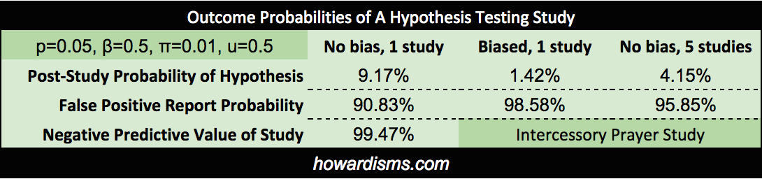
Two more examples. First, let’s apply this first step to the previously mentioned retrospective prayer study. The author used a p value of 0.05 as a cut off for statistical significance and there was no power analysis, so we might assume the study was under-powered, with a beta of 0.5. We might also assume significant bias in the construction of the study (u=0.5). Lastly, how likely do we think that prayer 10 years in the future will affect present-day outcomes? Let’s pretend that this has a 1% chance of being true based on available data. We find that the positive predictive value of this study is only 1.42%, if our bias assumption is correct, and no better than 9.17% if there were no bias, p-hacking, or other manipulations of any kind.
When you read about this study, you knew already in your gut what Bayes tells you clearly: There is an incredibly low chance, despite a well-designed and clinically significant trial, published in a prestigious journal, that the hypothesis is much more likely than the 1% probability we guessed in the first place. Note that it is slightly more likely than your pretest probability, but still so unlikely that we should not change our practices, as the author suggested.
We can use as a second example the BEAM Trial. Recall that this trial is the basis of using magnesium for prevention of cerebral palsy. We previously demonstrated that the findings of the trial were not statistically significant in the first place and are the result of p-hacking; but what if the results had been significant? Let’s do the analysis. We know that the p value used to claim significance for reduction of non-anomalous babies was p = 0.0491, so we can use this actual number in the calculations. The power of the trial was supposed to be 80% but the “significant” finding came in an underpowered subset analysis, so will set beta equal to 0.6. There were four previous studies which found no significant effect, so we will consider 5 studies in the field. Bias is a subjective determination, but the bias of the authors is clearly present and the p-hacking reinforces this. We will set bias to 0.4. Lastly we must consider what the probability of the hypothesis was prior to the study. Since four prior studies had been done which concluded no effect, the probability that the alternative hypothesis was true must be considered low prior to the trial; in fact, prior data had uniformly suggested increased neonatal death. Let’s be generous and say that it was 10%. What do we get?
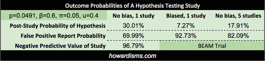
Since this was the fifth study (with the other four showing no effect), then the best post-study probability is 17.91%; that number doesn’t discount for bias. Incorporating the likely bias of the trial would push the PPV even lower, to about 3%. Of course, all of that assumes that the trial had a statistically significant finding in the first place (it did not). The negative predictive value, then, is the most precise number, which stands at 96.79%.
Either way, it is probably safe to say that as the data stands today, there is only about a ~3% chance that magnesium is associated with a reduced risk of CP in surviving preterm infants. Recall that Bayesian inference allows us to continually revise our estimate of the probability of the hypothesis based on new data. Since BEAM was published, two additional long-term follow-up studies of children exposed to antenatal magnesium have been published which showed no neurological benefit from the exposure in school-aged children. With Bayesian updating, we can use this data to further refine the probability that magnesium reduces the risk of cerebral palsy. If the estimate was ~3% after the BEAM Trial, it is now significantly lower based on this new information.
While we are discussing magnesium, how about its use as a tocolytic? Hundreds of studies have shown that it is ineffective, with at least 16 RCTs. What if a well-designed study were published tomorrow that showed a statistically-significant effect in reducing preterm labor? How would that change our understanding? With the overwhelming number of studies and meta-analyses that have failed to show an effect, let’s set the pre-study probability to about 1%:
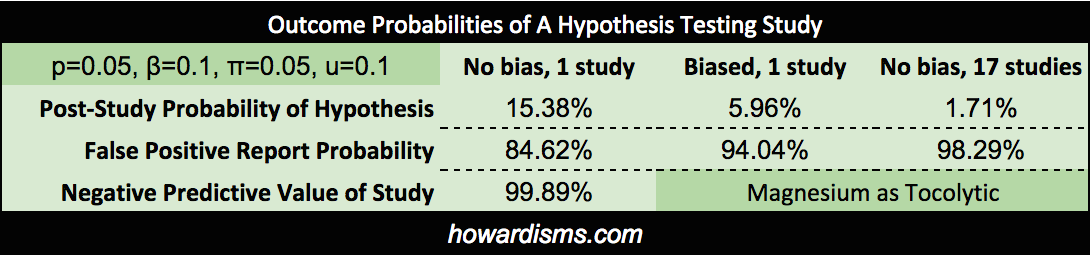
So just counting the RCT evidence against magnesium as a tocolytic, a perfectly designed, unbiased study would have no more than a 1.71% positive predictive value. A potential PPV so low means that such a study should not take place (though people continue to publish and research in this dead-end field). Bayesian inferences tells us that the belief that magnesium may work as a tocolytic or to prevent cerebral palsy has roughly the same evidence as the idea that remote intercessory prayer makes hospital stays of ten years ago shorter.
Here’s the general concept. Let’s graphically compare a high probability hypothesis (50%) to a low probability one (5%), using both an average test (lower power with questionable p values or bias) and a really good study (significant p value and well-powered).
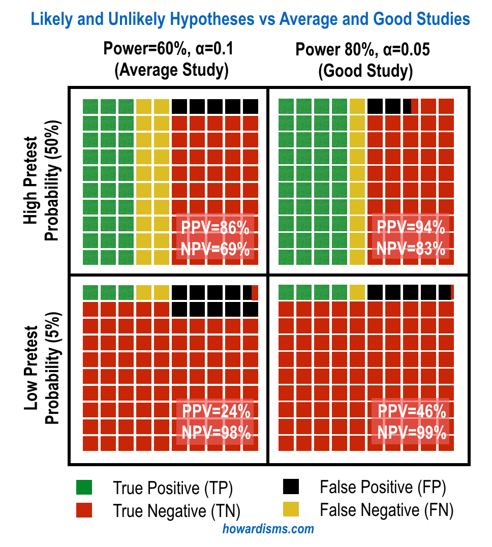
Take a look at the positive and negative predictive values; they are clearly influenced by the likelihood of the hypothesis. Many tested hypotheses are nowhere near as likely as 5%; the hypotheses of most epidemiological studies and other “data-mining” type studies may carry more like a 1 in 1,000 or even 1 in 10,000 odds.
3. Rejecting the Null Hypothesis Does Not Prove the Alternate Hypothesis
The casual view of the P value as posterior probability of the truth of the null hypothesis is false and not even close to valid under any reasonable model, yet this misunderstanding persists even in high-stakes settings. – Andrew Gellman
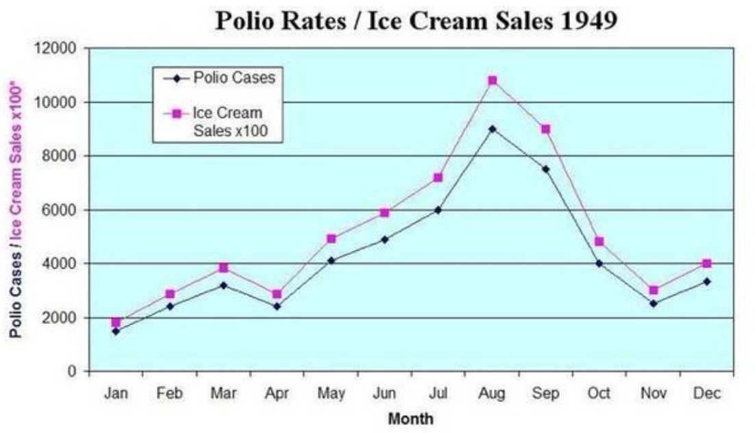
When the null hypothesis is rejected (in other words, when the p value is less than 0.05), that does not mean that THE alternative hypothesis is automatically accepted or that it is even probable. It means that AN alternative hypothesis is probable. But the alternative hypothesis espoused by the authors may not be the best (and therefore most probable) alternative hypothesis. For example, I may hypothesize that ice cream causes polio. This was a widely held belief in the 1940s. If I design a study in which the null hypothesis is that the incidence of polio is not correlated to the incidence of ice cream sales, and then I find that it is, then I reject the null hypothesis. But this does not then mean that ice cream causes polio. That is one of many alternative hypotheses and much more data is necessary to establish that any given alternative hypothesis is probable.
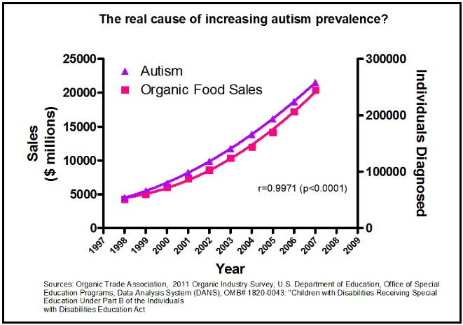
This is a mistake of “correlation equals causation” and this is the most likely mistake with this type of data. I’m fairly sure that organic foods do not cause autism though the two are strongly correlated (but admittedly, I could be wrong):
A study published just this week revealed a correlation between antenatal Tylenol use and subsequent behavioral problems in children. Aside from the fact that this was a poorly controlled, retrospective, epidemiological study (with almost no statistical relevance and incredibly weak pretest probability), even if it were better designed and did indeed determine that the two factors were significantly correlated, it still would be no more evidence that Tylenol causes behavioral problems in children than the above data is evidence that organic food causes autism. There are a myriad of explanations for the correlation. Perhaps mothers who have more headaches raise children with more behavioral problems? Or children with behavioral problems cause their mothers to have more headaches in their subsequent pregnancies? Correlation usually does not equal causation.
But if a legitimate finding were discovered, and it appears likely that it is causative, we must next assess how big the observed effect is.
4. Is the magnitude of the discovered effect clinically significant?
There are an almost endless number of discoveries that are highly statistically significant and probable, but they fail to be clinically significant because the magnitude of the effect is so little. We must distinguish between what is significant and what is important. In other words, we may accept the hypothesis after these first steps of our analysis, but still decide not to make use of the intervention in our practice.
I will briefly mention again a previous example: while it is likely true that using a statin drug may reduce a particular patient’s risk of a non-fatal MI by 1%age point over ten years, is this intervention worth the $4.5M it costs to do so (let alone all of the side effects of the drug)? I’ll let you (and your patient) decide. Here is a well-written article explaining many of these concepts with better examples. I will steal an example from the author. He says that saying that a study is “significant” is sometimes like bragging about winning the lottery when you only won $25. “Significant” is a term used by Frequentists whenever the observed data is below the designated p value, but that doesn’t mean that observed association really means anything in practical terms.
5. What cost is there for adopting the intervention into routine practice?
Cost comes in two forms, economic and noneconomic. The $4.5M cost of preventing one nonfatal MI in ten years is likely not to be considered cost-effective by any honest person. But noneconomic costs come in the form of unintended consequences, whether physical or psychological. Would, for example, an intervention that decreased the size of newborns by 3 ounces in mothers with gestational diabetes be worth implementation? Well, maybe. That 3 ounces might, over many thousands of women, save a few shoulder dystocias or cesareans. So if it were free, and had no significant unintended consequences, then yes it probably would be worth it. But few interventions are free and virtually none don’t expose the patients to unintended harms. So the cost must be worth the benefit.
Studies do not always account for all of the costs, intended and unintended. So often the burden of considering the costs of implementation fall upon the reader of the study. Ultimately, deciding whether to use any intervention is a shared decision between physician and patient and one which respects the values of the patient. The patient must be fully informed, understanding precisely both the risks and the benefits in terms she can understand.
Was Twain Right?
Many are so overwhelmed by the seemingly endless problems with scientific papers that the Twain comment of “Lies, Damned Lies, and Statistics” becomes almost an excuse to abandon science-based medicine and return to the dark ages of anecdotal medicine. Most physicians have been frustrated by some study that feels wrong but they can’t explain why it’s wrong, as the authors shout about their significant p value.
But Twain’s quote should be restated: There are lies, damned lies, and Frequentism. The scientific process is saved by Bayesian inference and probabilistic reasoning. Bayes makes no claim as to what is true or not true, only to what is more probable or less probable; Bayesian inference allows us to quantify this probability in a useful manner. Bayes allows us to consider all evidence, as it comes, and constantly refine how confident we are about what believe to be true. Imagine if rather than reporting p values, scientific papers concluded with an assessment of how probable the reported hypotheses are. This knowledge could be used to directly inform future studies and draw a contrast between Cigarettes and Elvis. But for now we must begin to do this work ourselves.
Criticisms
Why are Frequentists so resistant to Bayesian inference? We will discuss this in later posts; but, suffice it to say, it is mostly because there seems to be a lot of guessing about the information used to make these calculations. I don’t really know how likely it is that listening to Elvis causes brain cancer. I said 1% but, of course, it is probably more like 1 in a billion. This uncertainty bothers a lot of statisticians, so they don’t want to use a system that is dependent on so much uncertainty. Many statisticians are working on methods of improving the processes for making these calculations, which will hopefully make our guesses more and more accurate.
Yet, the fact remains that the statistical methods that Frequentists want to adhere to just cannot provide any type of answer to the question, Does listening to Elvis cause brain cancer? So even a poor answer is better than no answer. I have patients to treat and I need to do the best I can today. Still, when trying to determine the probability of the Elvis hypothesis, I erred on the side of caution; by estimating even a 1% probability of this hypothesis, I remained open-minded. But even then, my study only said that there was a tiny chance that it did. If I’m worried about it, I can repeat the study a few times or power it better and get an even lower posterior probability. I am not though, so Don’t Be Cruel.
Oh, also remember this: the father of Frequentism, Fisher, pervertedly used his statistical methods to argue that cigarette smoking did not cause lung cancer – a fact that had been established by Bayesian inference.
Equations
Don’t keep reading below unless you really care about the math…
Power is defined as the probability of finding a true relationship, it it exists:
![]()
Similarly, the probability of claiming a false relationship is bound by alpha, which is the threshold that authors select for statistical significance, usually 0.05:
![]()
Recall the formula for determining the positive predictive value (PPV) is:

First, we need to determine how many true positives occur, and how many total positives occur. We must consider R, which is the ratio of true relationships to false relationships:
![]()
This can be based upon generalizations of the particular research field (such as genomics, epidemiology, etc.) or specific information already known about the hypothesis from previous evidence. This R ratio is the basis of the prior probability, that is, the probability that the alternative hypothesis is true: ![]()
This prior probability is calculated according to the formula,

We can therefore express the PPV either in terms of R:
![]() Or we can express the PPV in terms of π (see here for source):
Or we can express the PPV in terms of π (see here for source):

If a coefficient of bias is considered, the equation becomes (see here for derivation):

Selecting for the degree of bias is usually subjective, unless methods are used for estimating bias in particular fields or for particular subjects (the prevailing bias). If there have been multiple, independent studies performed, where n is the number of independent studies, not accounting for any bias, the equation becomes:  The False Positive Report Probability (FPRP) can be calculated simply as 1–PPV, or directly in the simple case in terms of π as:
